Visualizing Fluent Bit agent with Prometheus/Grafana

Introduction

In this post, we'll explore how you can use Fluent Bit in combination with Prometheus and Grafana to visualize the performance and behavior of the Fluent Bit agent. We'll start by explaining what Prometheus and Grafana are, and then dive into the details of how to set up and use these tools together.

Prometheus

Prometheus is a monitoring system that scrapes metrics from different sources and stores them in a time-series database. It offers a flexible query language and visualization tools for analyzing the data and is highly scalable.

Grafana

Grafana is an open-source platform for data visualization and analysis that offers various visualization options, such as graphs, tables, and dashboards. It has a powerful query language and can integrate with different data sources including Prometheus.

Why visualize Fluent Bit with Prometheus and Grafana?

Visualizing the work of Fluent Bit with Prometheus and Grafana could provide several benefits. Here are some of the key purposes that can benefit you by utilizing visualization:

a) Monitor the input data rate

With visualization, you can track the input data rate of Fluent Bit and ensure it is meeting your desired level of handling. Ideally, the input data rate should remain relatively constant.

b) Improve Visibility of Retries and Drops

By utilizing Prometheus and Grafana, you could track the number of retries and drops that occur while Fluent Bit is sending data. Retrying means that Fluent Bit failed more than once to send the data, and it is trying again after a certain amount of time. Dropping data means it has lost the data entirely, often because reaching the maximum number of retries allowed. The number of retries and drops should hopefully always be zero. Monitoring these can help detect issues early and prevent data loss.

Even besides these two, you could also check the buffer data amount that Fluent Bit is holding, and compare it with the machine’s capacity, etc. There are various parameters you could visualize through these platforms, but in this blog we will cover a) and b) with some exercises to start off with your visualization.

Now we will move on to some exercises to show you how to visualize these!

Exercises of visualizing using Prometheus/Grafana

We will move on to exercises to test and visualize the key purposes mentioned above.

During the exercises, Fluent Bit would collect data and send it to Fluentd. Prometheus would then retrieve the data from Fluent Bit, while Grafana would obtain the data from Prometheus for visualization purposes. All of these components would be running on a single virtual machine running Ubuntu. Prior to beginning, please ensure that you have already installed Fluent Bit, Fluentd, and Docker.

The initial step would be to set up the data stream explained above. Here are the files to get ready:

• flb.conf
  This would be the Fluent Bit configuration file. It collects Fluent Bit metrics and CPU data, to be sent to Fluentd and Prometheus.

[SERVICE]
    flush           1
    log_level       info

[INPUT]
    name            fluentbit_metrics
    tag             internal_metrics
    scrape_interval 2

[INPUT]
    name            cpu
    tag             fluentbit_cpu_usage
    interval_sec    5

[OUTPUT]
    Match                       *
    Name                        forward
    Host                        fluent-handson.demo.local
    Port                        50005
    Retry_Limit                 2
    Storage.total_limit_size    5g
    ## Networking
    net.connect_timeout         5
    net.keepalive               on
    net.keepalive_idle_timeout  10
    net.keepalive_max_recycle   0

[OUTPUT]
    name            prometheus_exporter
    match           *
    host            0.0.0.0
    port            2021

• fld_aggregator.conf
  This is the Fluentd configuration file, receiving data from Fluent Bit.

<source>
  @type forward
  port 50005
</source>

<match *>
  @type stdout
</match>

• prometheus.yml
  This is the yaml file for Prometheus. You could set options such as scrape interval and job name.

global:
  scrape_interval: 10s # Set the scrape interval to every 10 seconds. Default is every 1 minute.

# A scrape configuration containing exactly one endpoint to scrape:
# Here it's Prometheus itself.
scrape_configs:
  - job_name: 'fluentbit'
    static_configs:
            - targets: ['fluent-handson.demo.local:2021']

Before moving on to visualization, run these commands to create the data streamline.

1. Run Fluentd

fluentd -c fld_aggregator.conf

2. Run Fluent Bit

fluent-bit -c flb.conf

3. Run Prometheus
*Make sure that the file path in the command would match the path of the yaml file we created above.

docker run -p 9090:9090 -v /root/monitoring/prometheus.yml:/etc/prometheus/prometheus.yml prom/prometheus

4. Run Grafana

docker run -d -p 3000:3000 grafana/grafana-enterprise

With all above properly done, you should be able to access Prometheus and Grafana through a web browser. Try these two links to see if you could see them running:

1. “http://hostname:9090”
   This would be for Prometheus. Replace ‘hostname’ with your hostname.

2. “http://hostname:3000”
   This should bring you to Grafana. Replace ‘hostname’ with your hostname, and type admin/admin to log in.

If you have any errors occurring, try restarting your machine to improve the situation.

a) Monitoring the input data rate

Let’s move on to monitoring the first option, input data rate!

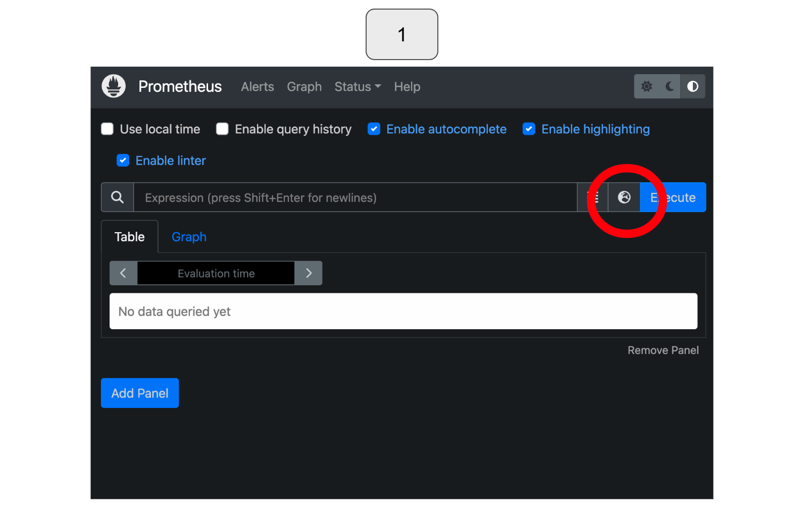
To visualize the input data rate, please follow the instructions provided below, which are also shown in the accompanying images with corresponding numbers.

1. In Prometheus, select the earth icon located in the top right corner.

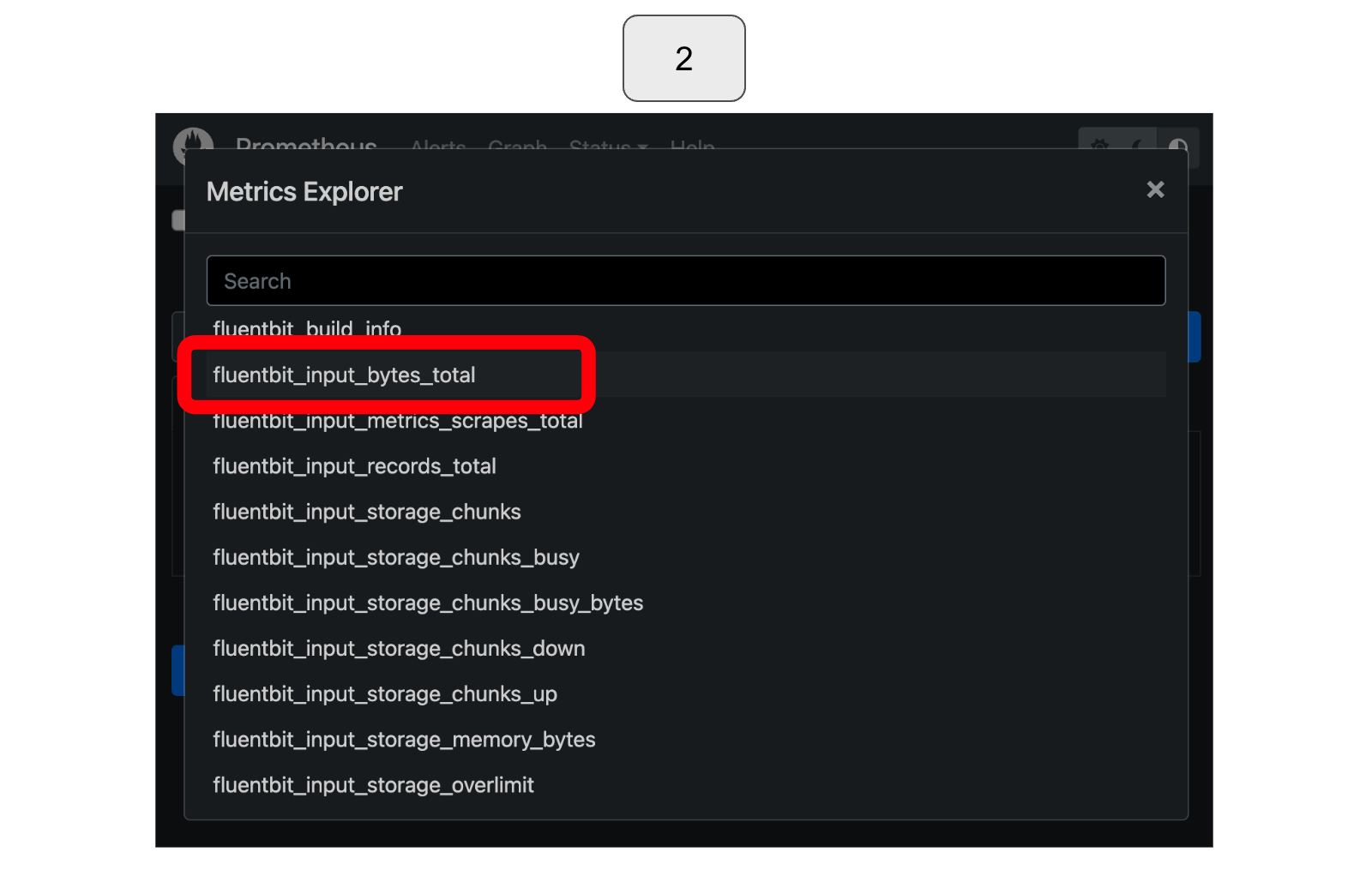
2. Within the available expressions for visualization, choose “fluentbit_input_records_total” as it corresponds to the input data rate we want to visualize.

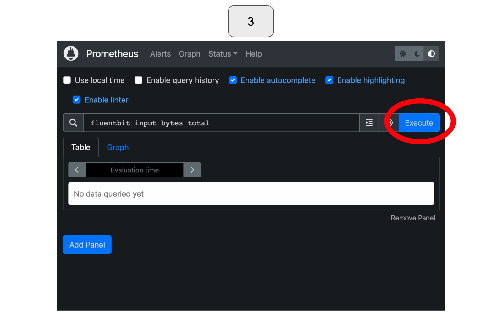
3. Once selected, click the blue “Execute” button in the top right corner.

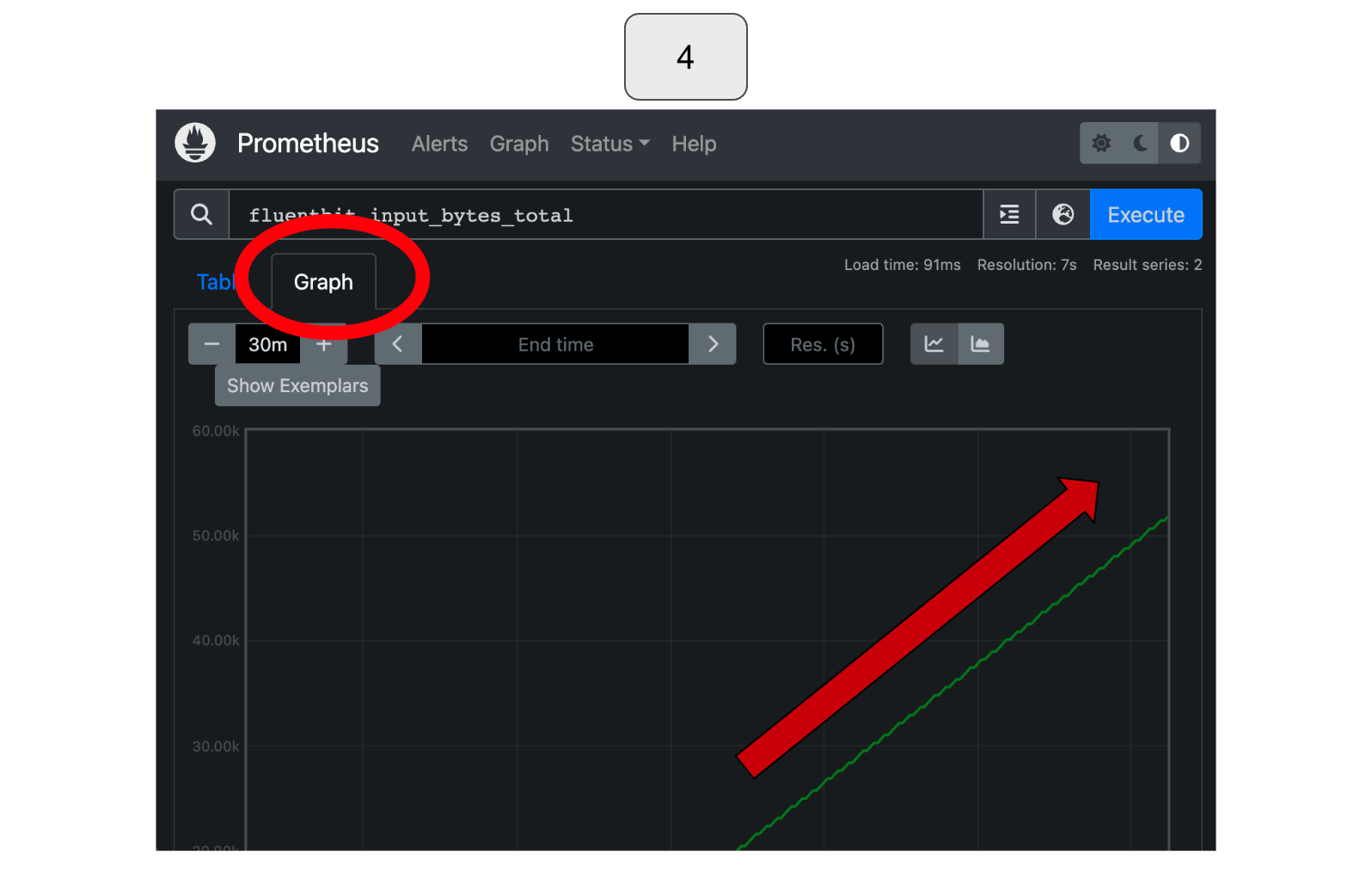
4. Select “Graph” and adjust the time range as necessary to observe changes in the total records. In this particular example, you would notice that the total amount of input data increases over time.

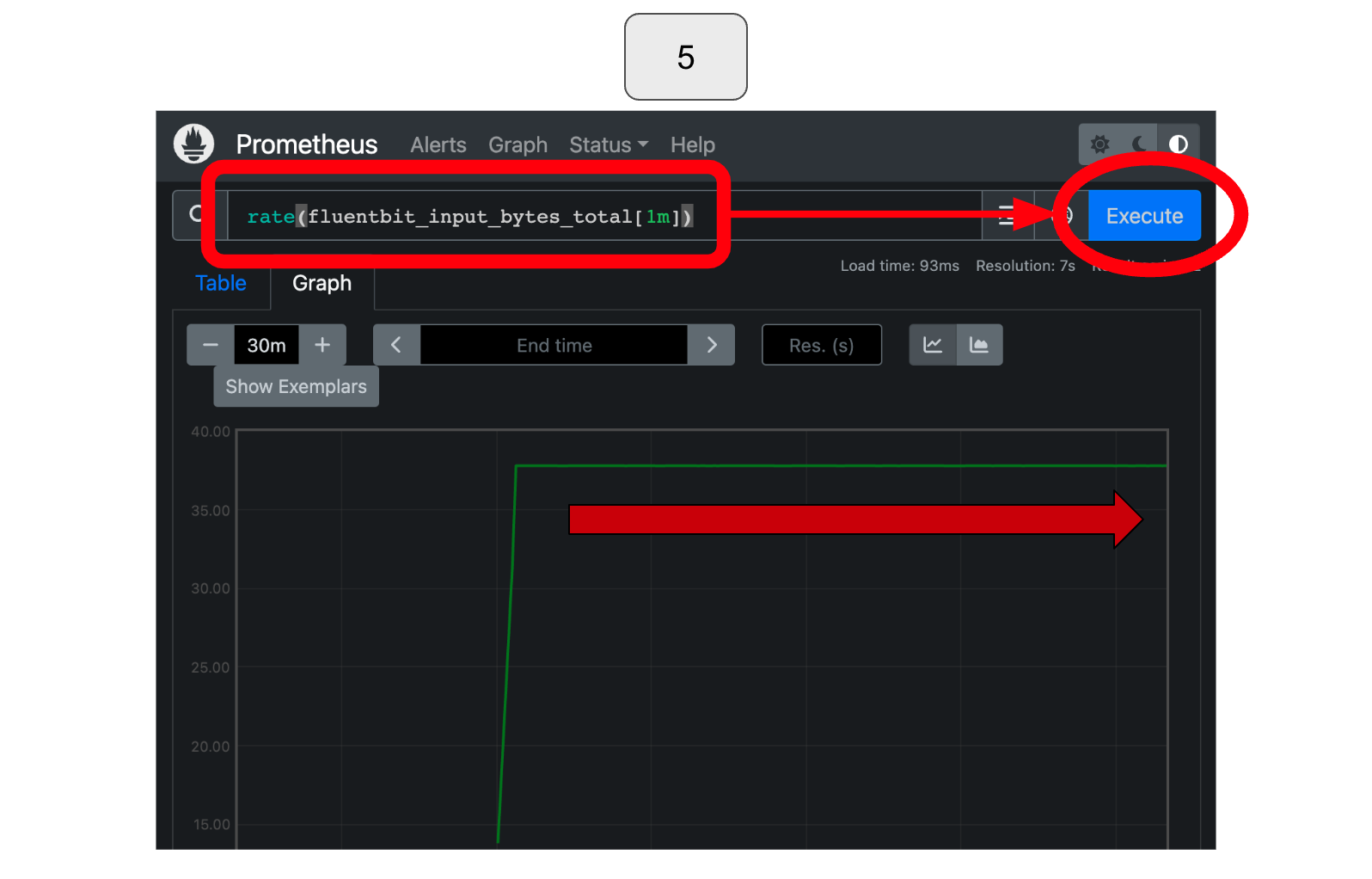
5. To check the input data rate, use the rate() function. For instance, in this example, you can observe the input records’ total amount per time over the last minute by using the expression “rate(fluentbit_input_bytes_total[1m])“. Based on this visualization, you can conclude that the input data rate is constant!

Let’s also work on visualizing with Grafana!

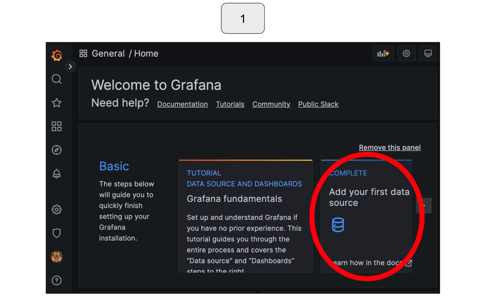
1. Starting from the Grafana icon in the top left corner, select “Add your first data source.”

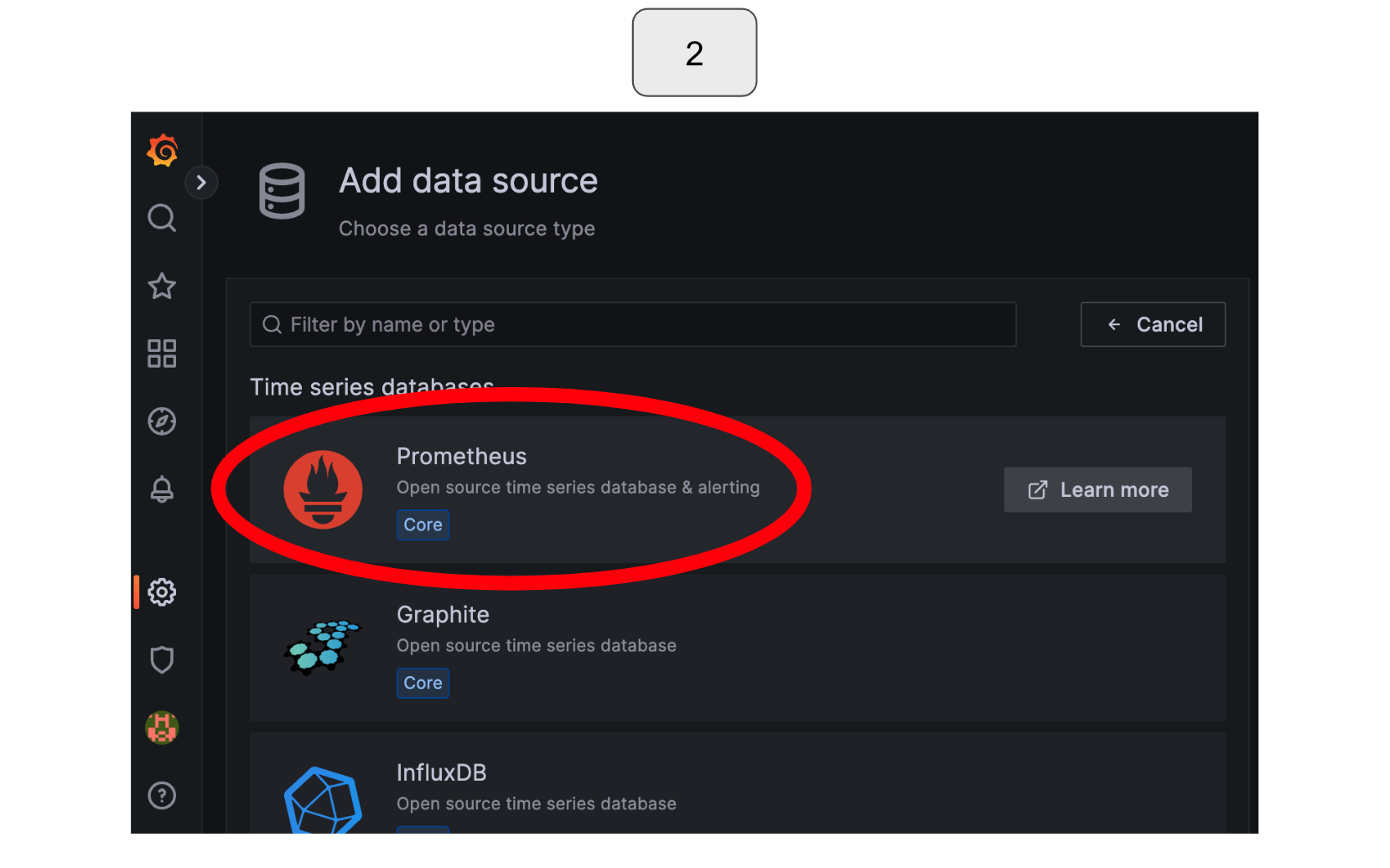
2. From the available options for data sources, select “Prometheus” for this exercise.

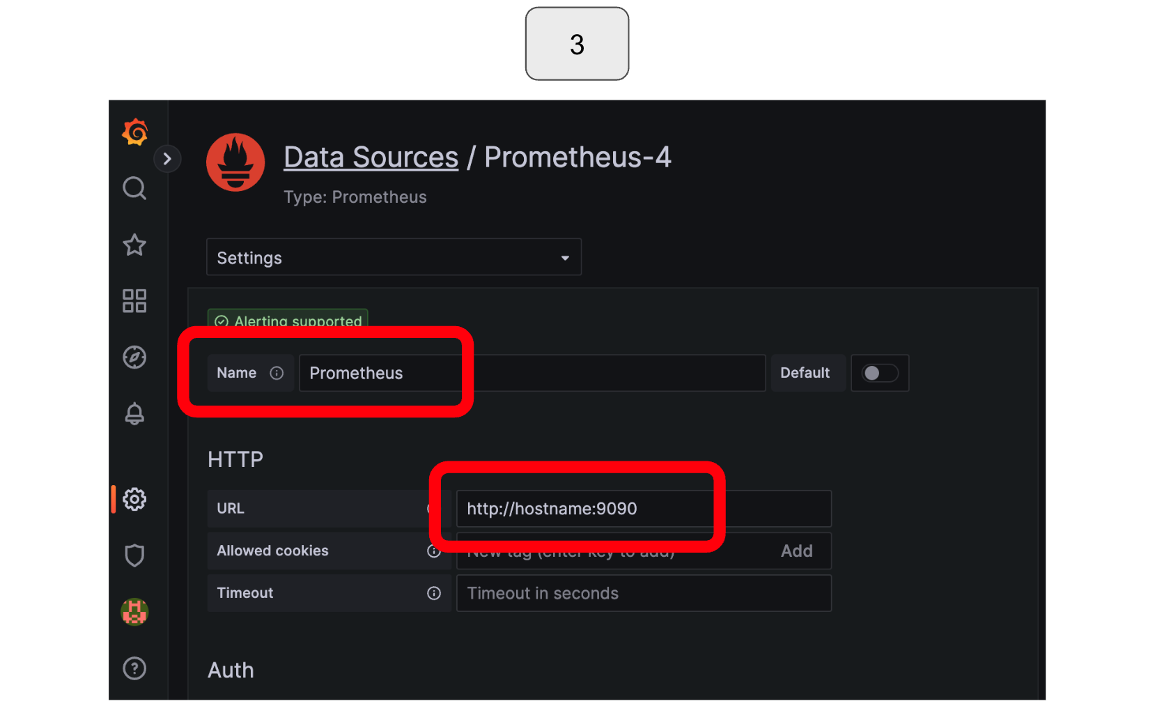
3. Enter the URL for your Prometheus server in the “URL” section.

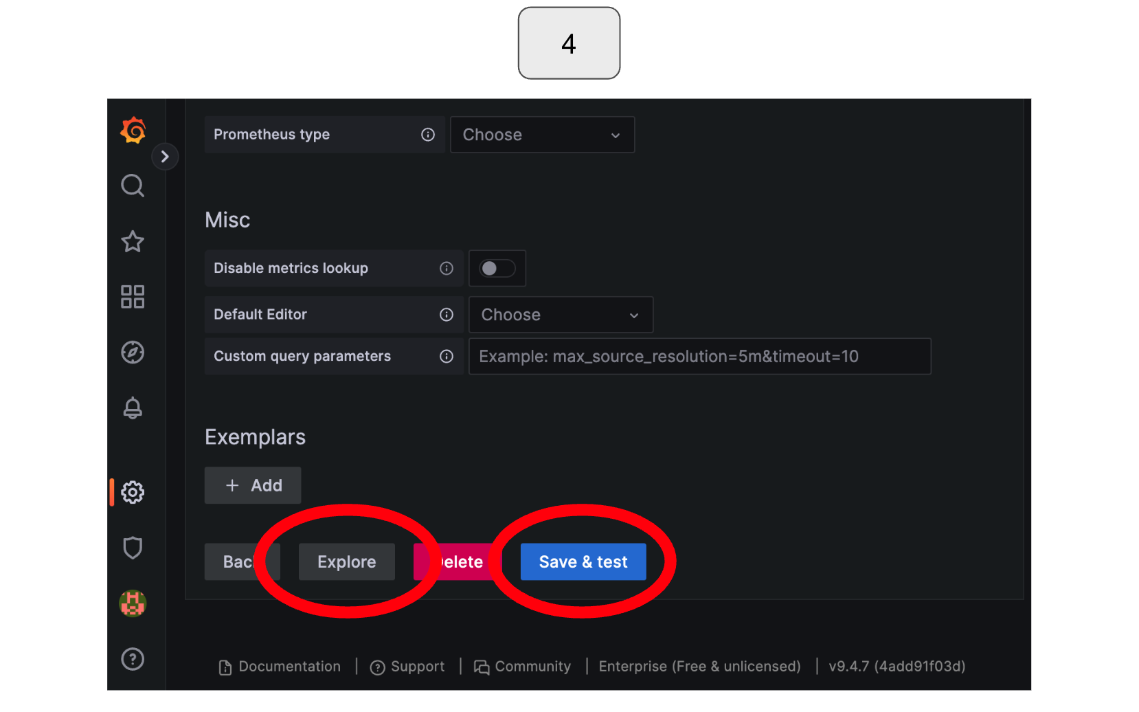
4. Scroll down to the bottom of the page and select “Save & Test,” followed by “Explore.”

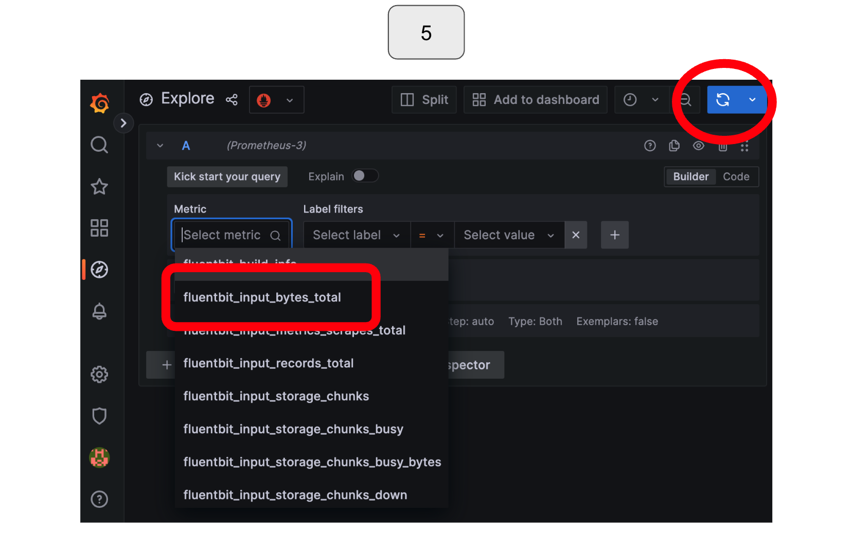
5. On the screen, select the “Metric” option on the screen and choose “fluentbit_input_records_total.” Run the query by clicking the blue button in the top right corner.

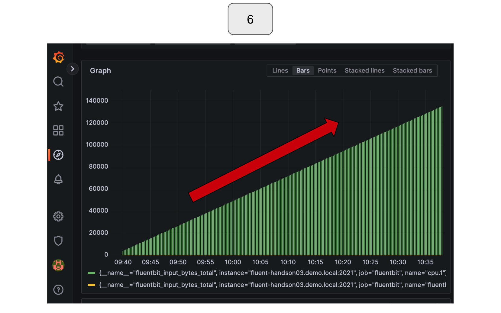
6. Observe how the input data is increasing.

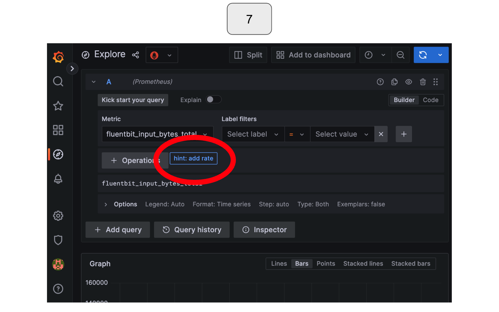
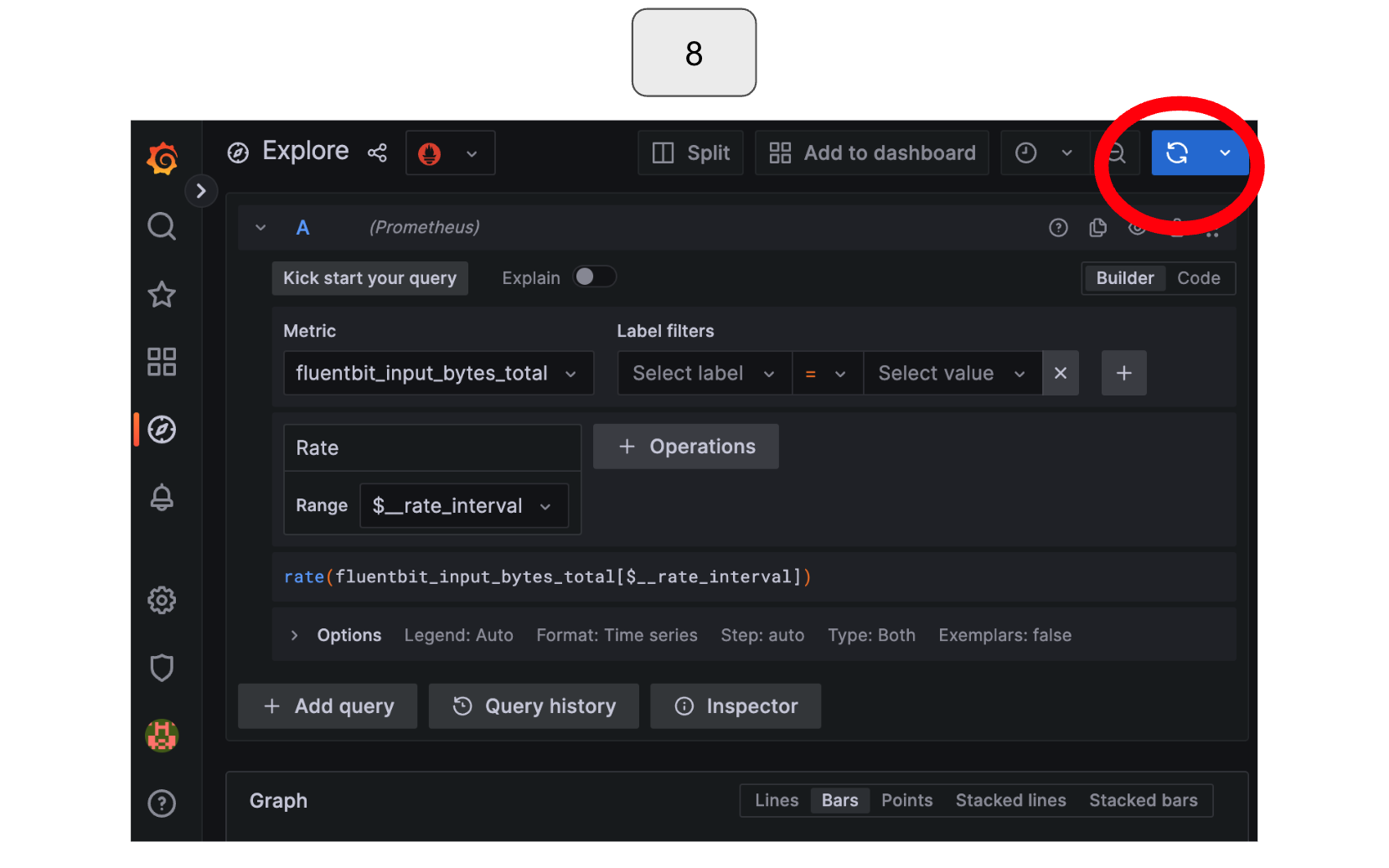
7. Click the “hint: add rate” button that appears below the metric options.

8. Run the query again.

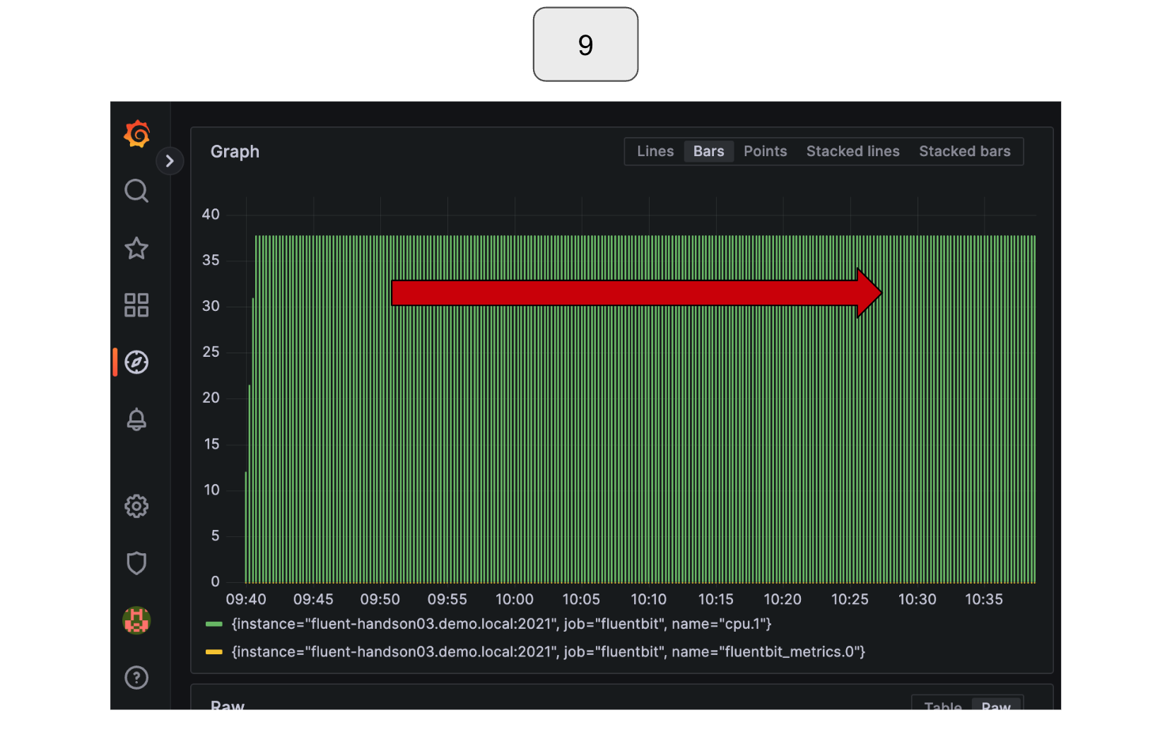
9. You should now be able to see a constant input data rate!

b) Improving Visibility of Retries and Drops

Next we will be checking the numbers of retries and drops of Fluent Bit. To intentionally create a failure to monitor these activities, we will briefly stop Fluentd. When Fluent Bit is unable to send data to Fluentd, it stores the data in a buffer and retries sending it later. Depending on the settings in the configuration file, Fluent Bit retries sending the data a certain number of times. If it is still unsuccessful in sending the data after reaching the maximum number of retries, it drops the data. You can observe how the numbers of retries and drops increase during these activities.

First, to stop Fluentd, open the terminal that you are running Fluentd and type ‘Ctrl’ + ‘C’ on your keyboard to interrupt the process. Wait for a few seconds or minutes, and then restart Fluentd. You may repeat these steps if you want.

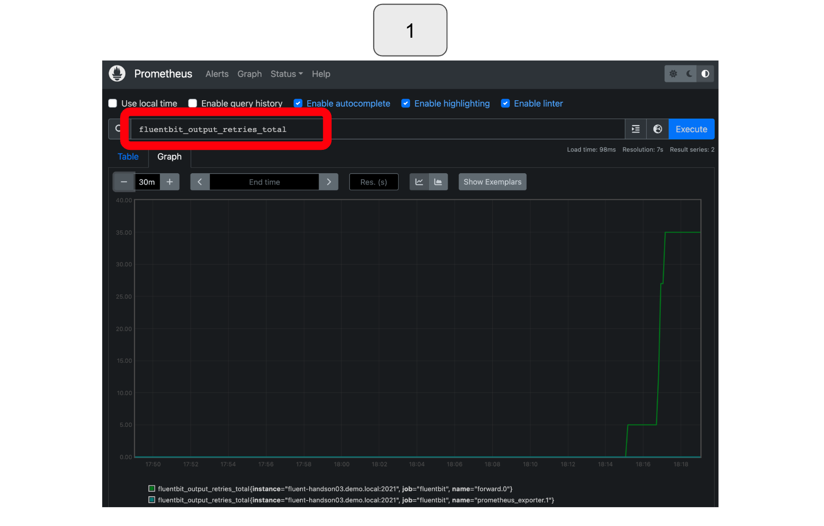
*In the example below, Fluentd was intentionally stopped twice, first for a shorter amount of time, and then for a longer duration. During the first stoppage, Fluent Bit attempted to resend the data several times and was successful before ultimately dropping it (retry counted but drop not counted). However, during the second stoppage, which lasted too long, Fluent Bit was unable to resend the data, resulting in data loss (retry and drop both counted).

After these activities,

1. In Prometheus, to monitor retries, select or type “fluentbit_output_retries_total.”

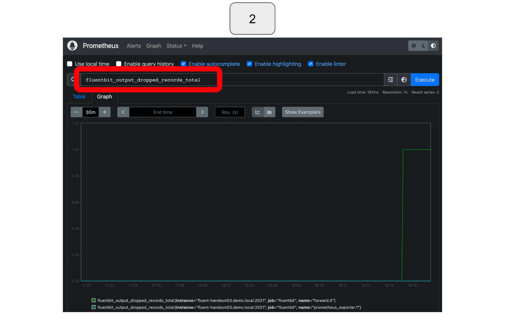
2. To monitor drops, select or type “fluentbit_output_dropped_records_total.”

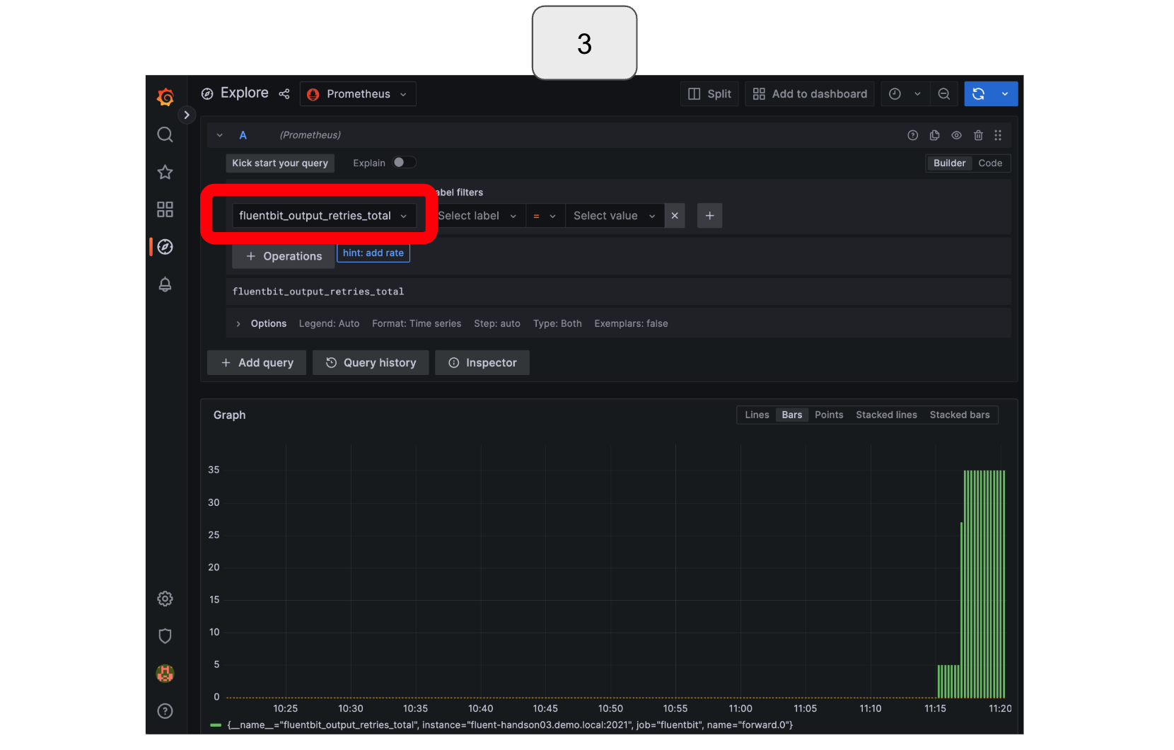
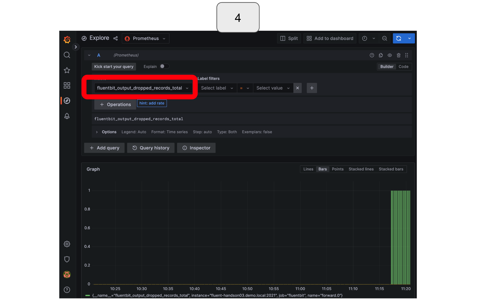
3. In Grafana, to monitor retries, select “fluentbit_output_retries_total.”

4. To monitor drops, select or type “fluentbit_output_dropped_records_total.”

Fantastic! You have now learned how to effectively visualize the key metrics using Prometheus and Grafana, as described in this blog post. There are countless other parameters you can visualize using these platforms, so feel free to experiment with them and deepen your knowledge. The specific parameters you can visualize depend on your configuration file and environment.

Need some help? - We are here for you.

In the Fluentd Subscription Network, we will provide you consultancy and professional services to help you run Fluentd and Fluent Bit with confidence by solving your pains. Service desk is also available for your operation and the team is equipped with the Diagtool and the knowledge of tips running Fluent Bit/Fluentd in production. Contact us anytime if you would like to learn more about our service offerings!